The Glass Box Transformer: A Language Model With the Lid Off
There is a moment in every explanation of a large language model where the explanation quietly stops.
It usually arrives about two-thirds of the way through, and it looks like a single line of code: loss.backward(). Everything up to that point has been described in loving detail — tokens, embeddings, queries and keys, the softmax, the residual stream. Then comes the backward pass, and instead of an explanation you get a method call. Behind that method call sits a recorded computation graph, a C++ dispatcher, a few thousand hand-optimised CUDA kernels, and a derivative rule for every operation you happened to use — all written by other people, years ago, and never once inspected by you.
I want to be clear that this is not a complaint about PyTorch. PyTorch is superb, and if you are building something real you should use it and not think twice. But if your goal is understanding rather than shipping, that line is a wall. You can build an entire career on the near side of it.
This article is about what is on the far side.
What follows is a complete walk through tinygpt.py — open it in a second tab and read along — a decoder-only transformer written in NumPy, in which every gradient is derived by hand and verified numerically. It has a byte-pair tokeniser, learned positional embeddings, causal multi-head attention, layer normalisation, a residual stream, Adam with bias correction, and temperature and nucleus sampling. Nothing has been omitted. Everything has simply been made small enough to see.
I have laid it out in the order the file executes, which is also the order in which the ideas depend on one another. Follow it to the end and you will have seen the complete lifecycle of a language model with no gaps papered over: text into numbers, numbers into a prediction, a prediction into a single measure of error, that one number into tens of thousands of individual corrections, and finally corrected numbers back into text.
And then, at the very end, I want to show you a formula that connects this file to GPT-3 with an error of less than one percent.
Part I — Two ways to write the same model
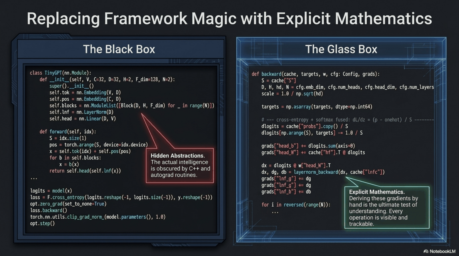
loss.backward() — behind which all of the interesting mathematics is hidden. On the right, the same computation with the gradients written out by hand. The left panel is what you should write at work. The right panel is what you should write once, in order to understand what the left panel is doing.Look at the left panel first. It is idiomatic, it is short, and it is completely opaque. nn.Embedding, nn.LayerNorm, nn.Linear, F.cross_entropy — each is a well-tested black box, and the model is assembled by naming them in the right order. Four lines then train it: compute the loss, zero the gradients, call backward, step the optimiser.
Now look at the right panel. def backward(cache, targets, w, cfg, grads). Everything the forward pass computed has been stashed in a cache, because the backward pass needs it. And every gradient is an explicit line of arithmetic that somebody had to derive on paper before they could type it.
Two lines in the middle of that panel are worth pointing at now, because we will spend a whole section on them later:
dlogits = cache["probs"].copy() / S
dlogits[np.arange(S), targets] -= 1.0 / S
That is the complete derivative of the loss with respect to the model's raw output scores. Two lines. Not two lines of calling something — two lines of arithmetic. When we derive it in Part VIII you will see why it is so short, and I think you will find the reason genuinely beautiful.
Here is the claim I want to defend across the rest of this article, and it is a claim about epistemics rather than engineering:
Which is exactly why, in Part X, we are going to prove the calculus correct by brute force.
The price of the glass box is about five hundred lines instead of forty, and a runtime slower by orders of magnitude — no GPU, no kernel fusion, no batching tricks. At twenty-eight thousand parameters that price is nothing. At twenty-eight billion it would be disqualifying. That is the honest trade, and it is why both panels exist.
Part II — The map
Before opening any single box, here is the whole file at once.
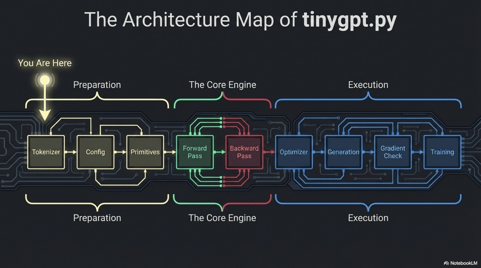
Preparation. The tokeniser converts text into integers, because a neural network is a function on numbers and cannot read. The config holds every size decision: two layers, thirty-two dimensional embeddings, two attention heads, a feed-forward block a hundred and twenty-eight wide, and a context window of thirty-two tokens. The primitives are the small mathematical utilities everything else stands on — layer normalisation, softmax, weight initialisation.
The core engine. The forward pass takes a sequence of token IDs and produces a probability distribution over what comes next, at every position. The backward pass takes the error in those distributions and converts it into a gradient for every parameter in the model. This is the transformer. Everything to its left is preparation; everything to its right is bookkeeping.
Execution. Adam applies the gradients. The gradient check proves the hand-derived calculus is right. Generation samples new text. The training loop runs the whole cycle a few thousand times.
Notice the proportions in that diagram, because they are not an artefact of this file being small. The core engine — the part that is actually the idea — is three boxes out of eleven. That ratio holds broadly at frontier scale too. The model is a comparatively small idea surrounded by an enormous amount of engineering, and when people describe modern AI as mostly infrastructure, this picture is what they mean.
Part III — The grain of the text
Every language model begins by confronting an awkward fact: a neural network is a function on numbers, and the word cat is not a number. Somebody has to solve that, and the two obvious solutions are both bad.
Give every word its own number, and the vocabulary explodes into the hundreds of thousands, most entries appear a handful of times, and the first time the model meets a word it has never seen — a surname, a typo, a drug name, a chemical formula — it is simply blind. Give every character its own number, and the vocabulary is tiny and nothing is ever unknown, but sequences become enormously long and the model burns its capacity relearning how to spell.
Byte-pair encoding is the compromise, and the clearest way to understand it is as greedy compression.
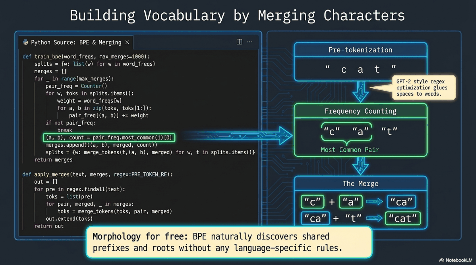
c and a merge into ca, then ca and t merge into cat. After enough rounds, common words are single tokens and rare words survive as fragments of familiar pieces.The entire learning rule of the tokeniser is one line, highlighted in the code panel:
(a, b), count = pair_freq.most_common(1)[0]
Whatever is most frequent, glue it together. That is the algorithm. Run it a thousand times — max_merges=1000 in the file — and a vocabulary precipitates out of the raw text.
Two details deserve attention. The first is the pre-tokenisation regular expression:
PRE_TOKEN_RE = re.compile(r"\s\w+|[^\w\s]") # GPT-2 style: space glued to word
Notice what that does: it deliberately attaches the leading space to the following word. So cat and ␣cat are two different tokens, with different IDs and different embeddings. This is not a quirk to be tidied away — it is the standard GPT-2 convention, and it is the reason these models are sometimes strangely sensitive to whitespace, and the reason the token count on your API bill is never your word count.
The second detail is the one I find genuinely striking, and it is the claim in the box at the bottom of the figure. Nobody told this algorithm that English has prefixes, suffixes, and roots. There is no linguistic knowledge anywhere in those fifteen lines. But because ing, un, and tion are statistically frequent adjacent pairs, they emerge as tokens in their own right. The tokeniser rediscovers a crude morphology of English purely by counting. Point the identical code at Japanese, at Python source, at protein sequences, and it will find the structure of those instead, with no modification at all.
rs in a word is like asking a colleague to count brushstrokes in a printed photograph — the information was discarded upstream, and no amount of capability downstream can recover it.
One last property worth stating: the mapping is lossless and reversible. apply_merges is deterministic, decoding is simple concatenation, and no information about the original string is destroyed. The tokeniser is a compression scheme, not a lossy summary.
Part IV — Keeping the arithmetic alive
This section is about plumbing. I am aware that plumbing sounds like the boring part. It is not: plumbing is where deep learning actually fails, and a meaningful share of the last decade's progress consists of people working out how to stop it failing.
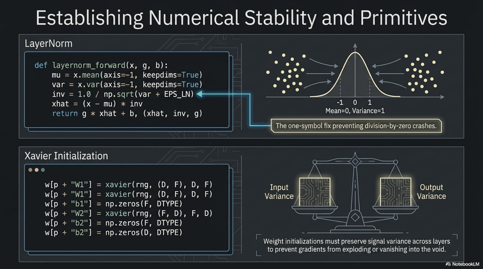
Layer normalisation is arithmetically trivial. Take a vector of thirty-two numbers, subtract its mean, divide by its standard deviation. It now has mean zero and variance one — precisely the picture on the right of the upper panel, scattered points pulled inward into a standard bell curve. Then multiply by a learnable gain g and add a learnable bias b, so the network retains the freedom to choose a different scale if it needs one.
Why do it at all? Because as signals pass through layers, their magnitude drifts. Drift upward and the numbers saturate or overflow. Drift downward and the gradients vanish into nothing. Normalising at every block holds the signal in the range where floating-point arithmetic is well-conditioned. More than any other single trick, it is the reason we can stack layers at all.
Now look at the annotation pointing at EPS_LN:
inv = 1.0 / np.sqrt(var + EPS_LN)
In this file, EPS_LN = 1e-5. If a vector happens to be constant — every element identical — its variance is exactly zero, and without that epsilon you have divided by zero. The result is NaN, which then propagates silently through every subsequent operation, contaminates the entire model, and never raises an error. The loss becomes nan, the run is dead, and nothing tells you where it started.
Xavier initialisation solves the same class of problem at the other end of the timeline. We start with random weights — but not just any random weights:
limit = np.sqrt(6.0 / (fan_in + fan_out))
return rng.uniform(-limit, limit, size=shape)
The purpose is the balance scale in the lower right of the figure: make the variance of a layer's output match the variance of its input. Initialise too large and activations grow multiplicatively layer after layer until they explode; too small and they shrink geometrically until no usable gradient survives back to the early layers. Note also that the biases start at exactly zero — there is no symmetry in a bias that needs breaking, so there is nothing to be gained by randomising it.
The general point, which I think the public hears far too rarely: a neural network is not robust magic. It is a numerically delicate computation that works only inside a fairly narrow band, and keeping it inside that band is a substantial part of the engineering.
Part V — What, where, and the wall against the future
We now have integers and stable arithmetic. Time to build the input the transformer actually consumes, which one line does almost entirely:
x = w["tok_emb"][ids] + w["pos_emb"][:S]
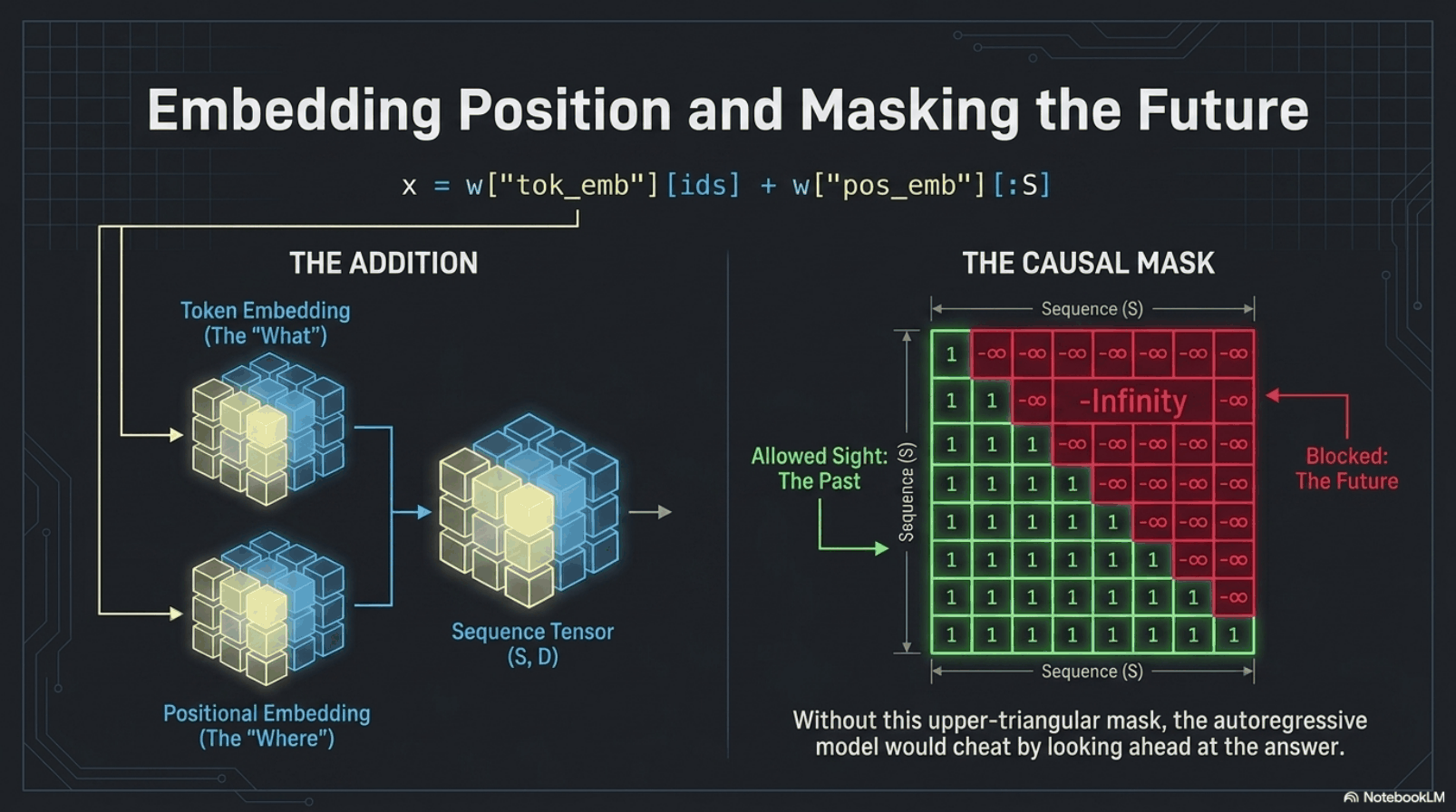
The token embedding is a lookup table. Each token ID indexes a row of thirty-two learned numbers. Those numbers are not assigned by anyone; they are learned, and over training, tokens appearing in similar contexts drift toward similar vectors. All of the famous word-vector geometry is a consequence of the prediction objective, not something anybody designed. This is the "what".
The positional embedding is a second table, indexed not by which token but by where it sits — position zero, one, two. This is the "where", and it is not optional. Attention, as we are about to see, is fundamentally a set operation with no built-in notion of order. Without positional information, "dog bites man" and "man bites dog" are literally the same input.
What surprises people is the plus sign. We do not concatenate the what and the where; we add them, into a single thirty-two dimensional vector. Intuitively that should destroy information — you cannot un-add two numbers. But in thirty-two dimensions there is ample room for the two signals to occupy near-orthogonal directions, and the network learns to keep them separable. Modern systems have largely moved to rotary embeddings, which rotate rather than add, but the purpose is identical.
The causal mask is the right-hand panel, and it solves a problem created by our own efficiency. We are training the model to predict the next token at every position simultaneously — that is what makes training tractable. But if we feed the entire sequence in at once, position three can see position seven, and position seven is the answer. The model would learn to copy rather than predict, drive the loss to almost zero, and generate nothing useful whatsoever. It is a spectacular bug, and an instructive one.
So before the softmax we add a matrix that is zero on and below the diagonal — the green region, the past, permitted — and negative infinity above it.
That single triangular matrix is what makes the model autoregressive. It is also the origin of a tension we will return to at the very end: it lets us train on every position in parallel, and it forces us to generate one token at a time, forever.
Part VI — What "paying attention" actually means
Let me define attention in one sentence before showing any code, because it is considerably simpler than its reputation.
Every position produces three vectors. A query — what am I looking for. A key — what do I have to offer. And a value — what I will contribute if you choose me. Every position compares its query against every key by taking a dot product; those scores are softmaxed into weights; and each position takes a weighted average of all the values, with weights proportional to how well its query matched each key.
That is attention. That is the entire mechanism. When someone says a model "pays attention" to a word, this is the literal operation: a dot product, a softmax, a weighted average. There is nobody inside doing the attending.
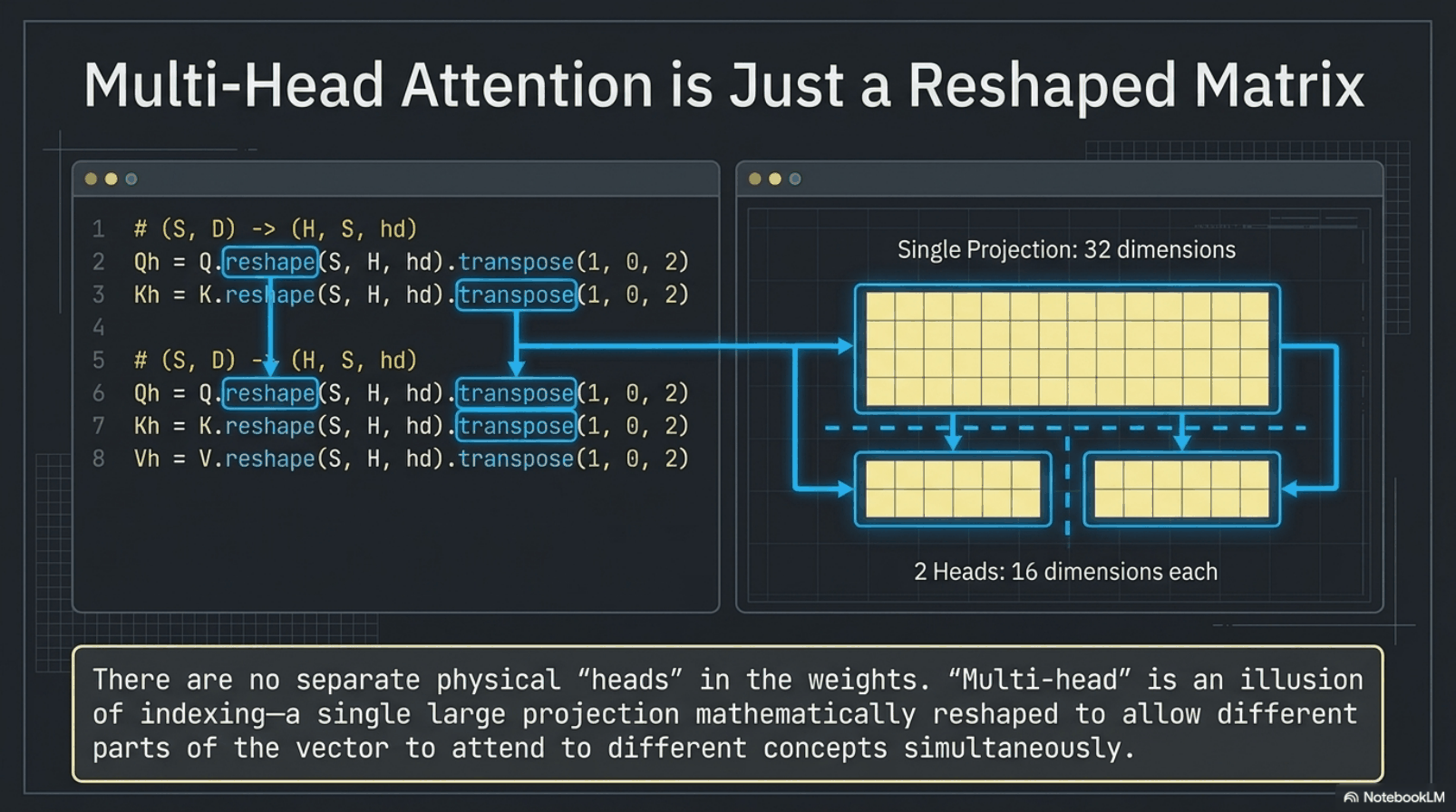
reshape and transpose here are views onto the same numbers.This is the point of the figure, and it is the thing most explanations get subtly wrong. "Multi-head attention" sounds like the model runs several independent copies of the machinery side by side. It does not. It is an illusion of indexing.
# (S, D) -> (H, S, hd)
Qh = Q.reshape(S, H, hd).transpose(1, 0, 2)
Kh = K.reshape(S, H, hd).transpose(1, 0, 2)
Vh = V.reshape(S, H, hd).transpose(1, 0, 2)
With D = 32 and H = 2, the head dimension hd is 16. Those three lines create no parameters. They change how the same block of memory is read.
So why bother? Because a dot product across all thirty-two dimensions yields exactly one attention pattern per position. Splitting into two sixteen-dimensional subspaces lets one head learn local syntactic adjacency while the other tracks a longer-range dependency — simultaneously, in the same forward pass, at essentially the same cost. Real models do this with thirty-two, sixty-four, or ninety-six heads. It is the cheapest expressiveness in the architecture.
One detail with outsized importance: the scale factor of one over the square root of the head dimension — here, one over four. Dot products between higher-dimensional vectors grow in magnitude with dimension. Left unscaled, the scores get large, the softmax saturates into a near one-hot spike, its gradient collapses toward zero, and the model stops learning. Dividing by sqrt(head_dim) holds the scores in a workable range. It is the same species of fix as the epsilon in Part IV, and equally invisible until it is missing.
Part VII — The stream and the funnel
Two plus signs on the left of the next figure represent, arguably, the most important structural idea in deep learning after the layer itself.
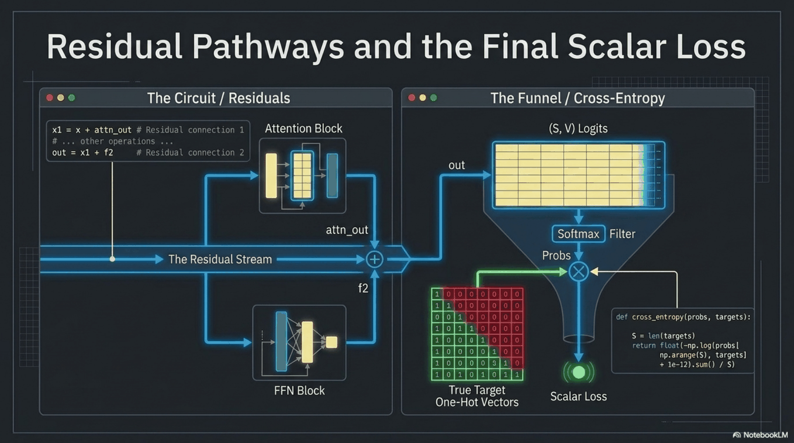
x1  = x + attn_out    # residual connection 1
out = x1 + f2         # residual connection 2
The metaphor in the figure is exactly right: the residual stream is a bus running the length of the model. Each block does not replace the representation — it reads the stream, computes a correction, and adds that correction back. Nothing is overwritten. If a block has nothing useful to contribute for a particular input, it can output approximately zero and the signal passes through untouched.
That has two large consequences. First, gradients. Because the path from output back to input contains an unbroken chain of additions, the derivative always carries a term equal to one, all the way down. Gradients cannot vanish the way they did in deep networks before around 2015. More than anything else, this is what made real depth possible. Second, interpretability. Because the stream persists, a feature written by an early layer can be read by a much later one — which is the mental model essentially all current interpretability research is built on.
The feed-forward block does something complementary to attention. Attention mixes information across positions; the FFN processes each position independently — expanding thirty-two dimensions up to a hundred and twenty-eight, applying a nonlinearity, projecting back down to thirty-two. The intuition I find most useful is that attention decides what to combine, and the feed-forward network decides what to make of it. In frontier models this block holds roughly two-thirds of all parameters.
Then the funnel. After a final layer normalisation, the output head projects each position's thirty-two numbers into V numbers, one per vocabulary token. Those are the logits — raw, unnormalised scores. Softmax converts them into a probability distribution. And cross-entropy does something almost embarrassingly simple:
def cross_entropy(probs, targets):
    S = len(targets)
    return float(-np.log(probs[np.arange(S), targets] + 1e-12).sum() / S)
Look up the probability the model assigned to the token that actually came next. Take the negative logarithm. Average over positions. That is the whole objective.
Sit with the shape of that funnel for a moment. Tens of thousands of parameters, an entire sequence, every attention pattern, every feed-forward computation — and it all collapses into one number. That scalar is the model's complete opinion of its own performance, and driving it downward is the only thing training does.
Two footnotes. The + 1e-12 inside the logarithm is the same defensive epsilon from Part IV, for the same reason: the log of zero is negative infinity. And the choice of the negative logarithm is not arbitrary — it punishes in proportion to confidence. Assign 0.9 to the correct token and you pay about 0.11. Assign 0.001 and you pay about 6.9. Being confident and wrong is expensive, which is precisely the incentive you want in a forecaster.
Part VIII — The spark
Here the backward pass begins, and this is the pivot of the whole article.
We need the derivative of the loss with respect to the logits — the raw scores, before softmax. Written out honestly, it is unpleasant. You are differentiating the logarithm of a softmax, and the derivative of softmax is not a number but a matrix, the Jacobian, because nudging any single logit changes every probability — they are constrained to sum to one, so they cannot move independently.
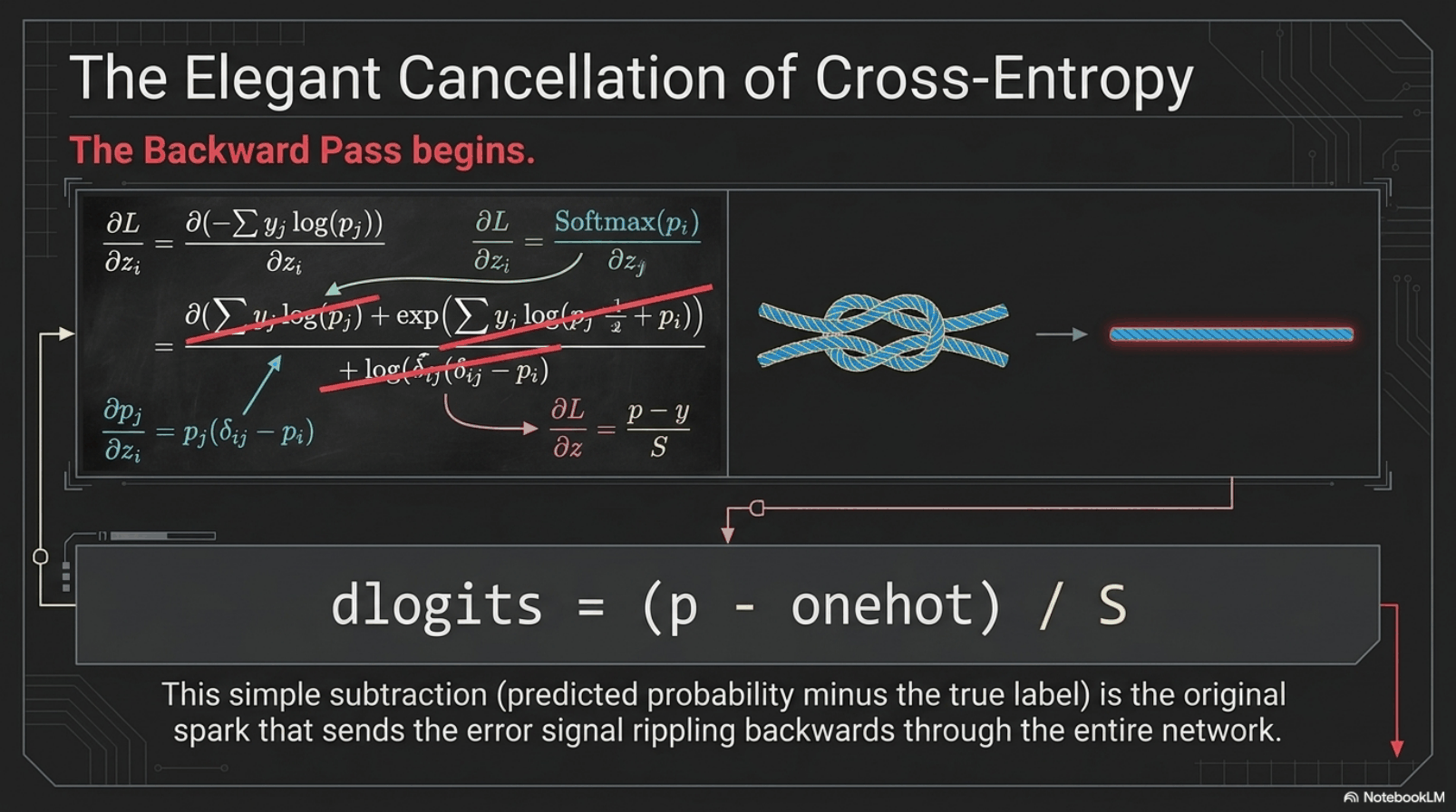
What survives the cancellation is this:
dlogits = (p - onehot) / S
Let me read that in plain English, because it deserves it. The gradient is the predicted probability minus the true label. If the model said seventy percent and that token was what came next, the error on that logit is −0.3. If it said seventy percent for a token that did not occur, the error is +0.7. The gradient is literally how wrong you were, with a sign attached.
This matters practically for two reasons. It is numerically stable — there is no division by a small probability anywhere, which the naive two-step formulation cannot avoid. And it is cheap: one subtraction. This is exactly why softmax and cross-entropy are always implemented as a single fused operation in every serious framework. They are not really two steps; separating them throws away the cancellation and buys you an instability for the privilege.
But it matters far more conceptually.
For those who work in this area: this is also why label smoothing and training-time temperature are such surgical interventions. They modify y and z respectively, right here, at the single point where learning signal is created. Nothing else in the architecture has that property.
Part IX — Unrolling the chain rule
This is the most technical section of the article. If you are reading for the shape of the argument rather than the indices, the summary is: reversing a matrix multiplication means transposing it and multiplying again, and everything below is that rule applied repeatedly and carefully.
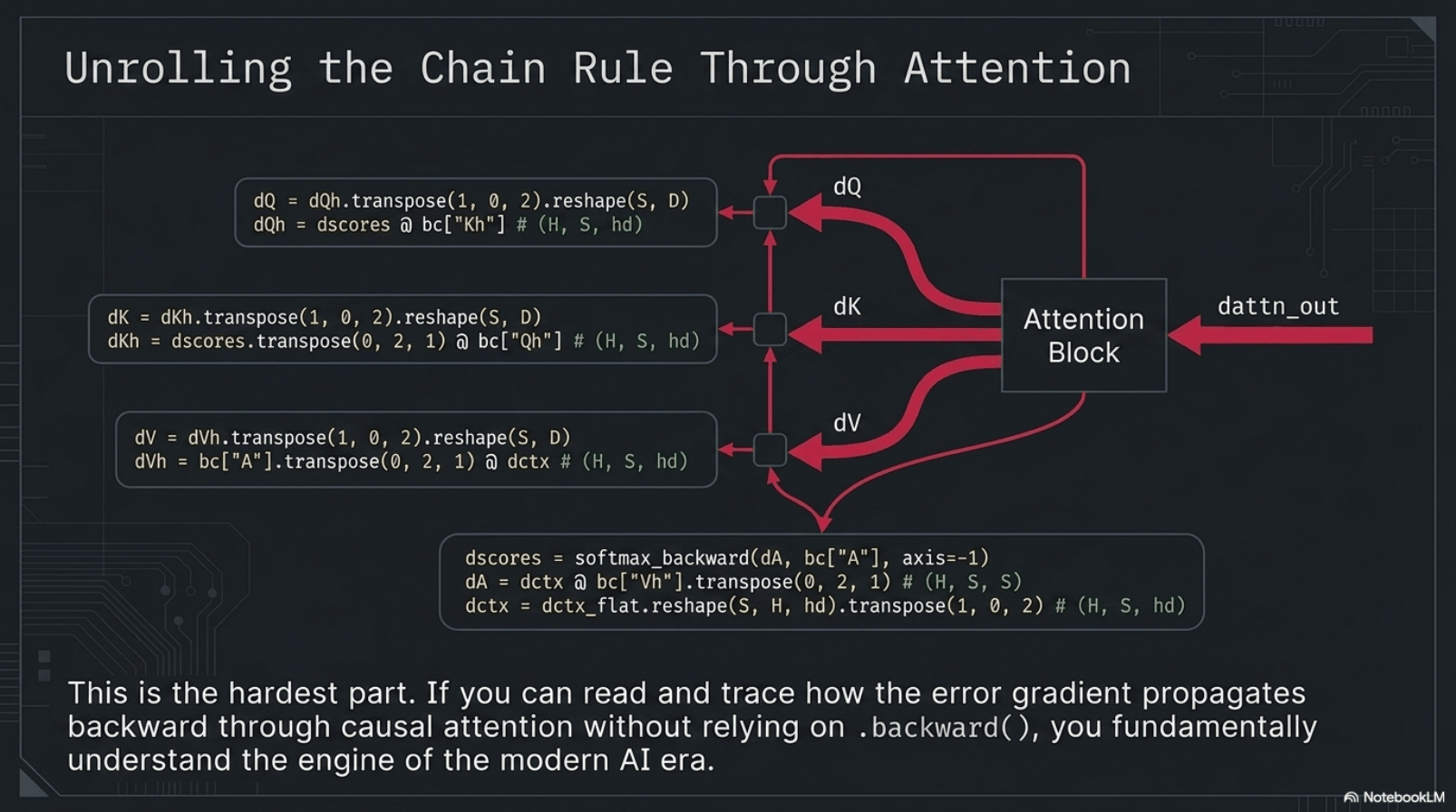
dattn_out, right) is decomposed into gradients for the value, key, and query projections, each of which must then be un-transposed and un-reshaped back into the layout the forward pass started from.The forward pass computed a context as attention weights times values, A @ Vh. So going backward, the gradient with respect to V is A.T @ dctx, and the gradient with respect to A is dctx @ V.T. Every matrix multiply in the forward pass becomes two matrix multiplies in the backward pass — which, incidentally, is why training costs roughly three times a forward pass, and why training budgets are estimated the way they are.
softmax_backward is the same Jacobian we met in Part VIII. But here it does not cancel, because there is no cross-entropy sitting next to it to cancel against. It has to be computed properly. That contrast is worth stating explicitly: the elegance of the previous section was a happy accident of a specific pairing, not a general property of softmax.
Then the scores split into queries and keys. Because scores were Q @ K.T, the gradient dQ receives dscores @ K and dK receives dscores.T @ Q. Note the symmetry — queries and keys are mirror images of one another in the backward pass, which is a useful sanity check when debugging.
Finally, look at the first line of each box in the figure: transpose(1, 0, 2).reshape(S, D). Every view we took on the way in has to be un-taken on the way out. The two heads, which were only ever a relabelling of one vector, are reassembled into a single thirty-two dimensional gradient.
And one detail I find quietly lovely: the causal mask handles itself. The positions we set to negative infinity received exactly zero probability in the forward pass, so they receive exactly zero gradient in the backward pass. There is no special-case code for it anywhere. It falls out of the mathematics.
Part X — Momentum, and proving the calculus
Two things remain before the model can speak: apply the gradients, and establish that they are correct.
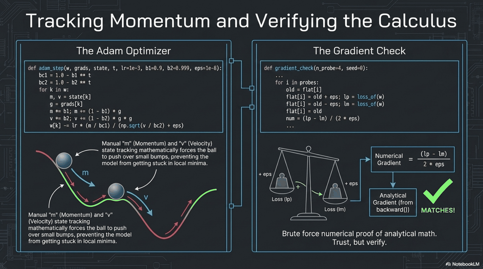
m, momentum) and of recent squared gradients (v, volatility), and divides one by the square root of the other. Right: the gradient check — nudge one parameter up and down by a tiny epsilon, measure the loss both times, and compare the resulting slope against what the analytical backward pass claimed.A raw gradient tells you which direction reduces the loss right now, for this batch. Following it directly is plain stochastic gradient descent, and it is jittery — it stalls on flat plateaus and oscillates across narrow valleys, exactly as the ball in the figure suggests.
Adam keeps two running averages for every single parameter. m is the average of recent gradients — momentum, the ball's accumulated velocity. v is the average of recent squared gradients — a measure of how volatile that parameter's gradient has been. The update divides m by the square root of v, so parameters whose gradients have pointed consistently in one direction take large, confident steps, while parameters that have been thrashing take small, cautious ones. In effect every parameter gets its own adaptively tuned learning rate.
The lines bc1 and bc2 are bias correction. Both averages start at zero, so early in training they are biased toward zero; dividing by one minus beta-to-the-power-t corrects it. It matters for roughly the first hundred steps and then becomes irrelevant — and it is exactly the kind of detail that is completely invisible inside torch.optim.Adam and completely visible here.
Now the right-hand panel, which is the part I would want a sceptic to look at.
We have written hundreds of lines of hand-derived calculus. How do we know any of it is right? We do not trust it. We test it. Take one parameter. Nudge it up by a tiny epsilon and measure the loss. Nudge it down by epsilon and measure again. The slope between those two points is the derivative — that is the definition of a derivative, and it requires no calculus at all, only two forward passes and the definition of a limit. Then compare it against what the analytical backward pass produced.
Running it on this file:
$ python tinygpt.py check
worst relative gradient error: 1.174e-08  (at b0.ln2_b[5])
PASS
Agreement to eight decimal places, in float64. The calculus is right.
And now the punchline, which is really the reason this entire field is computationally possible. Why not always compute gradients this way, and skip the derivations entirely? Because finite differences cost two full forward passes per parameter. For twenty-eight thousand parameters that is fifty-six thousand forward passes to obtain one training step's gradients. Backpropagation obtains all of them for the price of about two forward passes.
So we use brute force as a unit test on four randomly chosen parameters, and never as a method.
Part XI — What it actually does
It would be unsatisfying to walk through all of that and never show the thing running. So, a real training run on a small toy corpus:
$ python tinygpt.py train 300
vocab=21  sequences=67  params=27,861
uniform-baseline loss = ln(V) = 3.045

epoch    1  loss 3.5614  ppl  35.2  | 'the cat sat park a boy saw the dog queen a smiled
                                       the dog smiled on sat together the on park to saw'
epoch   50  loss 0.2917  ppl   1.3  | 'the cat sat on the mat together the girl ran to the
                                       park together the king saw the king saw the queen'
epoch  100  loss 0.1143  ppl   1.1  | 'the cat sat on the mat and the cat was happy the dog
                                       ran to the park and the dog was happy a boy saw the cat'
epoch  300  loss 0.1022  ppl   1.1  | 'the cat sat on the mat and the cat was happy the dog
                                       ran to the park and the dog was happy a boy saw the cat'
The progression is the point, and it recapitulates in three hundred epochs what pretraining does over months.
At epoch 1 the model has learned word frequencies and nothing else. Note that the loss, 3.56, is actually slightly worse than the uniform baseline of ln(21) = 3.045 — the random initialisation is worse than knowing nothing at all. The output has real words in plausible proportions and no structure whatsoever.
By epoch 50 the loss has fallen by an order of magnitude and the grammar has arrived, but the content is scrambled: "the king saw the king saw the queen". It has learned the shape of a sentence before it has learned which sentences exist.
By epoch 100 it reproduces the corpus. And it should — with 27,861 parameters and 67 training sequences, memorisation is the optimum. There is nothing to generalise to. Loss flattens at 0.10 and stays there.
That last point is worth being blunt about, because it is where small demonstrations are usually oversold: this model has not learned language. It has learned this corpus. What it demonstrates is that the mechanism works — that hand-derived gradients drive a real optimisation to a real optimum. Capability is a separate question, and it is a question about scale, which is where we finish.
Part XII — Choosing a word
Training is over. The model now hands us, for any context, a probability distribution over the entire vocabulary. And then a decision has to be made that is not part of the model at all.
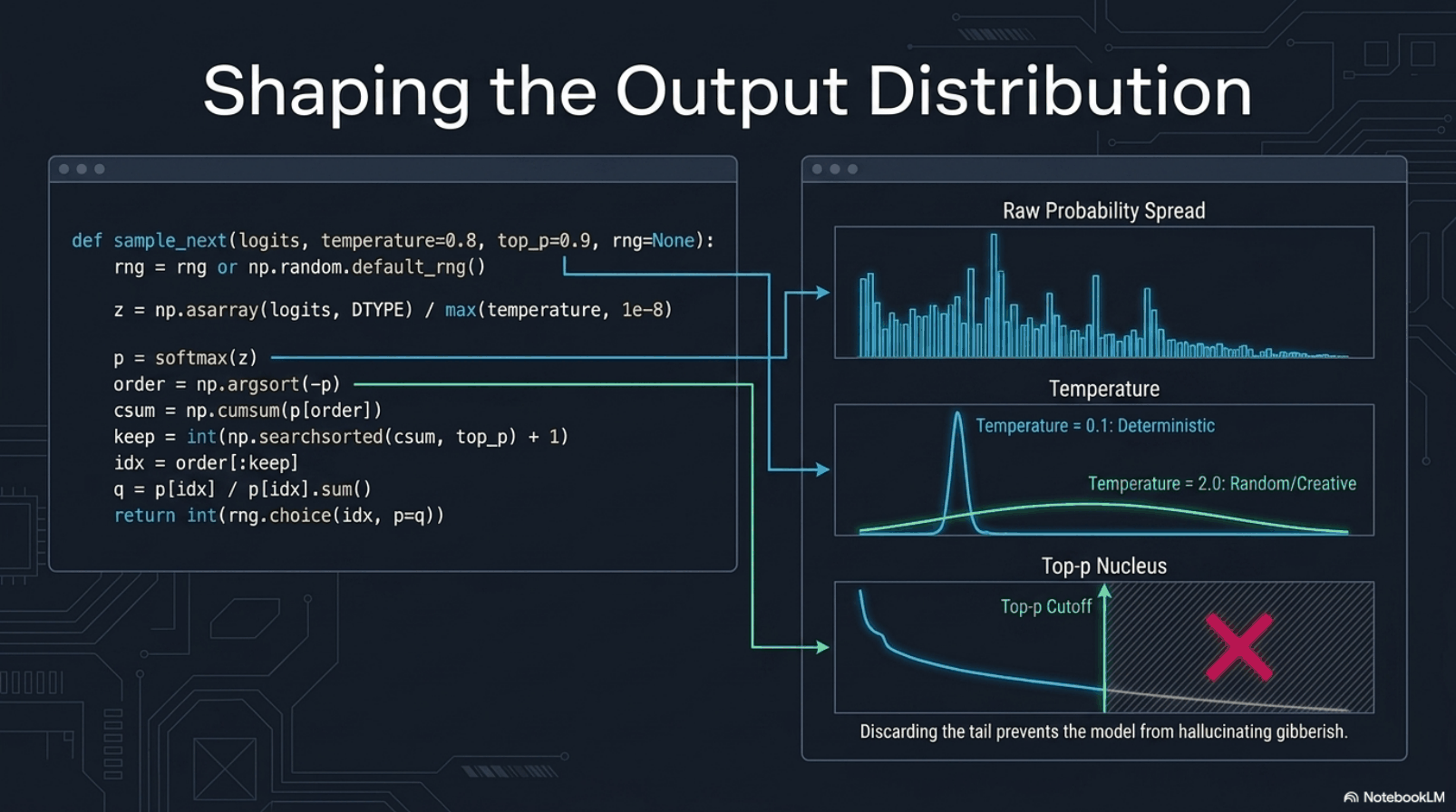
p and discards the shaded remainder entirely.The obvious answer — always take the highest-probability token — is called greedy decoding, and it produces repetitive, often degenerate text. Models fall into loops and repeat phrases indefinitely. It is worse than it sounds.
Temperature divides the logits by T before the softmax. Below one, the distribution sharpens toward determinism — safer, blander. Above one it flattens — more surprising, and considerably more likely to be nonsense. This file defaults to 0.8, slightly conservative.
z = np.asarray(logits, DTYPE) / max(temperature, 1e-8)
I want to state that plainly: temperature is one division. That is the entire mechanism behind the word "creativity" in every interface you have ever used.
Nucleus sampling, or top-p, is barely more complex. Sort the probabilities descending, accumulate until the running total reaches p — here 0.9 — keep those tokens, discard the rest, renormalise what remains.
Why does this matter more than it appears? Because the tail is enormous. Ten thousand tokens each carrying a probability of one in ten thousand collectively hold a substantial share of the distribution. Sample five hundred tokens in sequence and "occasionally absurd" becomes "reliably absurd". Nucleus sampling amputates that tail — and crucially, it does so adaptively. When the model is confident the nucleus may be one or two tokens; when it is genuinely uncertain it may be several hundred. The cutoff moves with the model's own confidence, which is why it outperforms a fixed top-k.
Part XIII — One blind step at a time
Four steps, repeated forever. This is generation, complete.
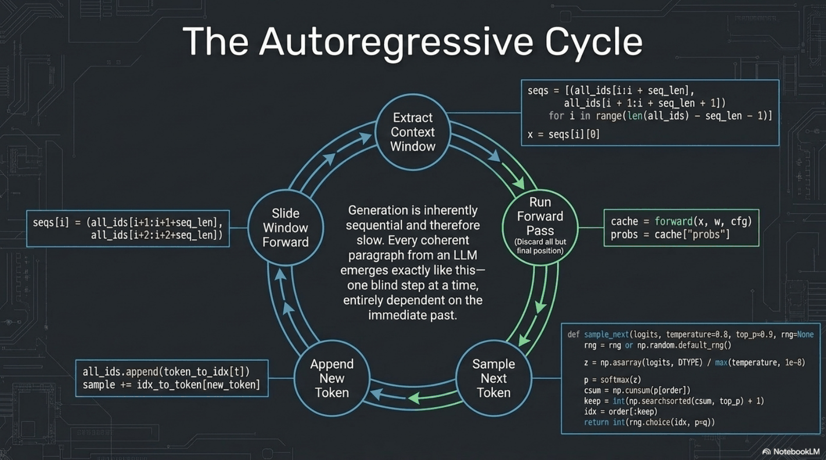
Pause on the wastefulness of step two. We compute predictions for all thirty-two positions and throw away thirty-one of them. Production systems fix this with a key-value cache — storing previous keys and values so each new token costs one position of work rather than an entire window — and it is the single most important inference optimisation there is. But the logic is exactly what the figure shows.
Now the sentence in the centre of that diagram, which is the one I would most want a general reader to take away. Generation is inherently sequential, and therefore slow. Training could be parallelised across every position at once — that is what the causal mask bought us in Part V. Generation cannot be. Token four hundred cannot begin to exist until token three hundred and ninety-nine does.
And here is what follows from that, which I think is underappreciated outside this field:
That single fact explains a surprising amount of observed behaviour. It explains why a model that commits to a wrong opening will sometimes confabulate elaborately to remain consistent with it — the opening is now part of its context, and context is all it has. It explains why "think step by step" works: it converts internal computation the model cannot perform into external tokens it can write down and re-read, using the page as working memory. And it explains why the last token of a long answer is produced with no more foresight than the first.
One further limit worth stating plainly: the model has no memory whatsoever beyond its window. Anything that has scrolled out of those thirty-two positions is gone — not compressed, not summarised, not retrievable. Frontier models have vastly larger windows, but the property is identical in kind.
Part XIV — Seven orders of magnitude
Which brings us to the only question that really matters about a file this small: is any of it different at a hundred and seventy-five billion parameters?
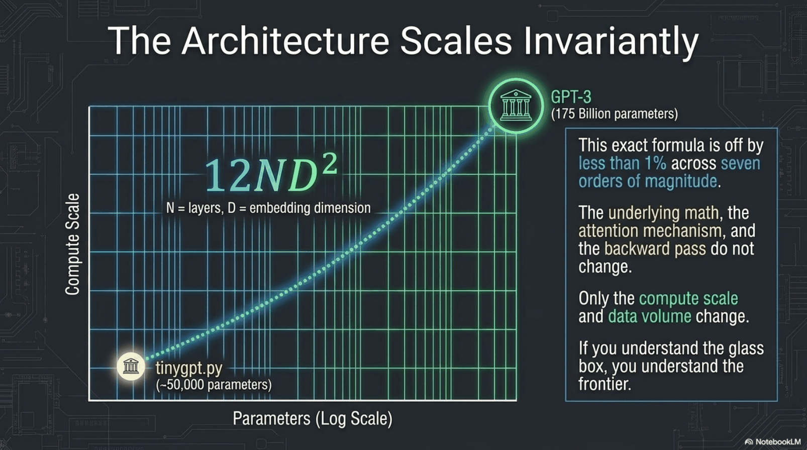
Check the formula at our end. Two layers, thirty-two dimensions: 12 × 2 × 32² = 24,576 non-embedding parameters. Add the embedding tables, the output head, and the normalisation gains and biases, and the file reports 27,861 for a twenty-one token vocabulary — the number in the training run above. Scale the vocabulary up and you reach the fifty thousand quoted on the title slide; the non-embedding core stays fixed at 24,576 regardless.
Now check it at the other end. GPT-3 has 96 layers and an embedding dimension of 12,288.
12 × 96 × 12,288² ≈ 173.9 billion. The published figure is 175 billion. An error of 0.6%, across seven orders of magnitude.
Let me state the conclusion without hedging. Nothing structural changed between those two dots. Not the attention mechanism. Not the residual stream. Not the derivative of cross-entropy. Not Adam, not the causal mask, not nucleus sampling. The file we have walked through is not a simplified analogy for a frontier model. It is the same object with different constants.
What did change is compute, data, and engineering: thousands of accelerators instead of one CPU, trillions of tokens instead of a text file, and an enormous body of genuinely difficult work in distributed training, data curation, and post-training alignment. I do not want to minimise any of that. It is where almost all of the effort and almost all of the money go. But it is not a different idea.
And now the caveat that intellectual honesty requires, because the argument above is easy to overstate and I have seen it overstated.
But here is what I hope you take from all of this.
The thing at the centre of the most consequential technology of this decade is not unknowable. It is a few hundred lines of arithmetic — tokenisation by counting, lookup tables, dot products, a softmax, some additions, a subtraction that carries the entire learning signal, and a great deal of patient bookkeeping. You have now seen all of it, with nothing hidden behind a method call.
The glass box is not a metaphor for the black box. It is the black box, at a size you can hold.
— Neal
tinygpt.py is a single self-contained file; NumPy is the only dependency. python tinygpt.py check runs the numerical gradient verification; python tinygpt.py train trains on a toy corpus and samples from it. The derivations discussed here, and the file itself, are also in how-llms-work-study.
Provenance. I wrote this NumPy port, and the hand-derived backward pass and gradient check that go with it, while working through CJ Reynolds' I Built an LLM from Scratch (Syntax), in which the same model is built in TypeScript. The architecture itself is from the literature — Vaswani et al. (2017), Radford et al. (2018), Ba et al. (2016), Kingma & Ba (2014), Glorot & Bengio (2010), Holtzman et al. (2019) — but the debt for the route through it is his.