Backpropagation has a reputation it does not deserve.
It is usually presented in one of two unhelpful ways. Either you get a page of symbols with superscripts in brackets and subscripts stacked two deep, which is precise and completely opaque. Or you get a friendly story about "errors flowing backwards through the network," which is comforting and tells you nothing you could act on.
The truth is that backpropagation is one small idea, applied repeatedly. The idea is:
If I nudge this number a tiny bit, how much does that number move?
That is it. Everything else — the chain rule, the layers, the sums, the matrices — is bookkeeping for asking that question efficiently about a few million numbers at once.
This post assumes you know no calculus at all. Not "rusty calculus." None. We will build what we need from scratch, and we will check every single claim with arithmetic you can do on paper. By the end you will have:
- worked a complete neural network forward and backward by hand, with real numbers;
- verified every derivative by nudging a number and watching what happens, so you never have to take a formula on trust;
- built the whole thing in a spreadsheet;
- and watched the network's error actually go down.
I have computed every number in this post and checked each derivative against a numerical nudge. They agree to about nine decimal places. If your arithmetic disagrees with mine, one of us has made a mistake and it is worth finding out which.
Part 0 — The three ideas, in advance
It helps to know where we are going.
Idea one: a derivative is a ratio of nudges. Not a limit, not a tangent line, not anything from a textbook. If I push this input up by a whisker and the output moves three whiskers, the derivative is 3. That is the whole definition we need.
Idea two: nudges multiply along a chain. If turning gear A by one tooth turns gear B by two teeth, and turning gear B by one tooth turns gear C by five teeth, then turning A by one tooth turns C by ten. This is the chain rule. It is multiplication, and it is not deep.
Idea three: we work backwards because it is cheaper. We want to know how every weight in the network affects one final number, the error. Starting from the error and working back lets us reuse almost all of the work. Starting from each weight and working forwards would mean redoing the same calculation thousands of times.
That is the entire post. What follows is those three ideas, slowly, with numbers.
Part 1 — What a derivative actually is
Forget everything you have heard about calculus. Here is a question anyone can answer.
I have a square tile with sides of length 3, so its area is 9. I make the side slightly longer — 3.01 instead of 3. What happens to the area?
New area: 3.01 × 3.01 = 9.0601.
The side went up by 0.01. The area went up by 0.0601. So the area moved about six times as much as the side did:
$$\frac{0.0601}{0.01} = 6.01$$
Let us make the nudge smaller. Side 3.001:
- new area = 9.006001
- area changed by 0.006001
- ratio = 6.001
Smaller still. Side 3.0001:
- ratio = 6.0001
You can see where this is heading. As the nudge gets smaller, the ratio settles down onto exactly 6.
That number — 6 — is the derivative of "area" with respect to "side," at side = 3. It is written \(\frac{dA}{ds}\), which you should read out loud as "how much A moves when I nudge s", and not as anything more mysterious.
Deriving it properly, with no calculus
We just found 6 by trying numbers. Let us get it exactly, using nothing but school algebra.
Call the side \(s\) and the nudge \(h\). The area is \(s^2\). After the nudge it is \((s+h)^2\). Multiply that out:
$$(s+h)^2 = s^2 + 2sh + h^2$$
So the change in area is
$$(s^2 + 2sh + h^2) - s^2 = 2sh + h^2$$
And the ratio of the change in area to the change in side is
$$\frac{2sh + h^2}{h} = 2s + h$$
Now look at that answer: \(2s + h\). The nudge \(h\) is something we get to choose, and we are choosing it smaller and smaller. As \(h\) shrinks towards nothing, the ratio settles on
$$\boxed{\frac{dA}{ds} = 2s}$$
At \(s = 3\) that gives \(2 \times 3 = 6\). Which is exactly what our arithmetic showed.
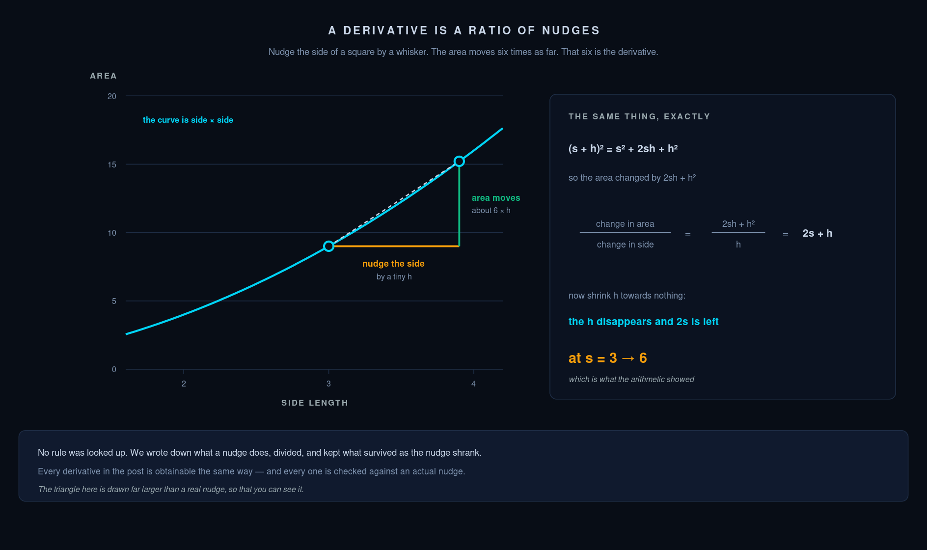
This is what "from first principles" means. We did not look up a rule. We wrote down what a nudge does, divided, and watched what survived when the nudge went to zero. Every derivative in this post is obtainable the same way, and you are entitled to be suspicious of any formula I give you until you have nudged it yourself.
We will use this exact result later, because the network's error will be a squared quantity.
The one piece of notation
I will write \(\frac{dC}{dw}\) to mean "if I nudge \(w\) a tiny bit, how many times more does \(C\) move?"
If \(\frac{dC}{dw} = -0.056\), it means: push \(w\) up by a small amount and \(C\) goes down by about 0.056 times that amount. The minus sign is direction, nothing more.
That is the only notation you need for the whole post.
Part 2 — The chain rule, from first principles
Here is the second idea, and it is the engine of the whole algorithm.
The exchange-rate version
Suppose you are converting money.
- 1 pound buys 1.3 dollars.
- 1 dollar buys 150 yen.
How many yen does a pound buy?
$$1.3 \times 150 = 195$$
Nobody finds this hard. You multiplied the rates. And note what a "rate" is here: it is exactly a ratio of nudges. "One more pound gets you 1.3 more dollars" is \(\frac{d(\text{dollars})}{d(\text{pounds})} = 1.3\).
So the chain rule — the thing that supposedly makes backpropagation difficult — is this:
$$\frac{d(\text{yen})}{d(\text{pounds})} = \frac{d(\text{yen})}{d(\text{dollars})} \times \frac{d(\text{dollars})}{d(\text{pounds})}$$
It is unit conversion. The middle quantity cancels the way units cancel, and that is not a coincidence.
Why it is true, not just plausible
Let us be careful, because "the symbols cancel" is a hint, not a proof.
Suppose \(u\) affects \(v\), and \(v\) affects \(w\). Nudge \(u\) by a tiny amount \(h\).
- \(v\) changes by approximately \(\frac{dv}{du} \times h\). Call that change \(k\).
- Now \(v\) has moved by \(k\), so \(w\) changes by approximately \(\frac{dw}{dv} \times k\).
Substitute:
$$\text{change in } w \approx \frac{dw}{dv} \times \left( \frac{dv}{du} \times h \right)$$
Divide both sides by \(h\) to get the ratio we want:
$$\frac{\text{change in } w}{h} \approx \frac{dw}{dv} \times \frac{dv}{du}$$
And as \(h\) shrinks to nothing, the approximations become exact:
$$\boxed{\frac{dw}{du} = \frac{dw}{dv} \times \frac{dv}{du}}$$
The word "approximately" is doing real work in the middle there, and making it rigorous is what a first-year analysis course is for. But the reason it works is the reason exchange rates work: over a small enough range, everything behaves like a straight line, and the slopes of straight lines multiply.
A numerical check, because you should not trust me
Let \(u = 2\). Let \(v = 3u\), so \(v = 6\). Let \(w = v^2\), so \(w = 36\).
By the chain rule: \(\frac{dw}{du} = \frac{dw}{dv} \times \frac{dv}{du} = (2v) \times 3 = 12 \times 3 = 36\).
Now nudge directly. Set \(u = 2.001\):
- \(v = 6.003\)
- \(w = 6.003^2 = 36.036009\)
- change in \(w\) = 0.036009
- ratio = \(0.036009 / 0.001 = 36.009\)
Which is 36, plus a little rounding from the nudge not being infinitely small. The chain rule holds.
Chains can be as long as you like. Four stages? Multiply four rates. This is the entire reason a hundred-layer network is not conceptually harder than a two-layer one — it is just a longer product.
Part 3 — The smallest possible network
Now we build something to differentiate.
Our network takes one number in and gives one number out. It has two layers. Here is the complete machine:
x ──[× w₁, + b₁]──→ z₁ ──[σ]──→ a₁ ──[× w₂, + b₂]──→ z₂ ──[σ]──→ a₂ ──→ compare to y ──→ C
Read left to right. In words:
- Take the input \(x\). Multiply by a weight \(w_1\), add a bias \(b_1\). Call the result \(z_1\).
- Squash \(z_1\) through a function \(\sigma\) to get \(a_1\). This is the hidden neuron's output.
- Multiply \(a_1\) by a second weight \(w_2\), add a second bias \(b_2\). Call it \(z_2\).
- Squash it again to get \(a_2\). This is the network's answer.
- Compare \(a_2\) to the correct answer \(y\), and score how wrong we were. That score is \(C\), the cost.
Written as five short equations:
$$z_1 = w_1 x + b_1 \qquad a_1 = \sigma(z_1) \qquad z_2 = w_2 a_1 + b_2 \qquad a_2 = \sigma(z_2) \qquad C = (a_2 - y)^2$$
Every one of those is a simple step. Multiply and add. Squash. Multiply and add. Squash. Square the mistake. There is nothing in a real neural network that is harder than this — there is only more of it.
The squashing function
\(\sigma\) (Greek letter sigma) is the sigmoid. Its job is to take any number at all and squash it into the range 0 to 1:
$$\sigma(z) = \frac{1}{1 + e^{-z}}$$
If that formula means nothing to you, it does not matter. All you need is that it turns big numbers into nearly 1, very negative numbers into nearly 0, and 0 into exactly 0.5. In a spreadsheet it is =1/(1+EXP(-z)).
For pencil work, here is a lookup table. These are the only values you need:
| \(z\) | \(\sigma(z)\) | \(z\) | \(\sigma(z)\) | |
|---|---|---|---|---|
| −2 | 0.1192 | 0.25 | 0.5622 | |
| −1.5 | 0.1824 | 0.5 | 0.6225 | |
| −1 | 0.2689 | 0.7311 | 0.6750 | |
| −0.5 | 0.3775 | 1 | 0.7311 | |
| −0.25 | 0.4378 | 1.14 | 0.7577 | |
| 0 | 0.5000 | 1.5 | 0.8176 |
Why a cost of \((a_2 - y)^2\)
We need a single number that says how wrong the network is, and it must be smallest when the network is right.
\((a_2 - y)^2\) does that. If the answer is perfect, \(a_2 - y = 0\) and the cost is 0. If we are wrong in either direction, squaring makes it positive, so being too high and being too low are both penalised. And squaring punishes big mistakes disproportionately — being wrong by 0.4 costs four times as much as being wrong by 0.2, not twice.
And here is the payoff from Part 1. We already know how to differentiate a square. We found \(\frac{d(s^2)}{ds} = 2s\) by expanding \((s+h)^2\). The same expansion, with \(s\) replaced by \((a_2 - y)\), gives us
$$\frac{dC}{da_2} = 2(a_2 - y)$$
We derived that ourselves in Part 1. We did not look it up.
Part 4 — The forward pass, by hand
Set up the problem. Pick these starting numbers:
| Quantity | Value | Meaning |
|---|---|---|
| \(x\) | 2.0 | the input |
| \(y\) | 1.0 | the correct answer |
| \(w_1\) | 0.5 | first weight |
| \(b_1\) | 0.0 | first bias |
| \(w_2\) | 1.0 | second weight |
| \(b_2\) | 0.0 | second bias |
The weights are made up. In a real network they start random. Now push the input through.
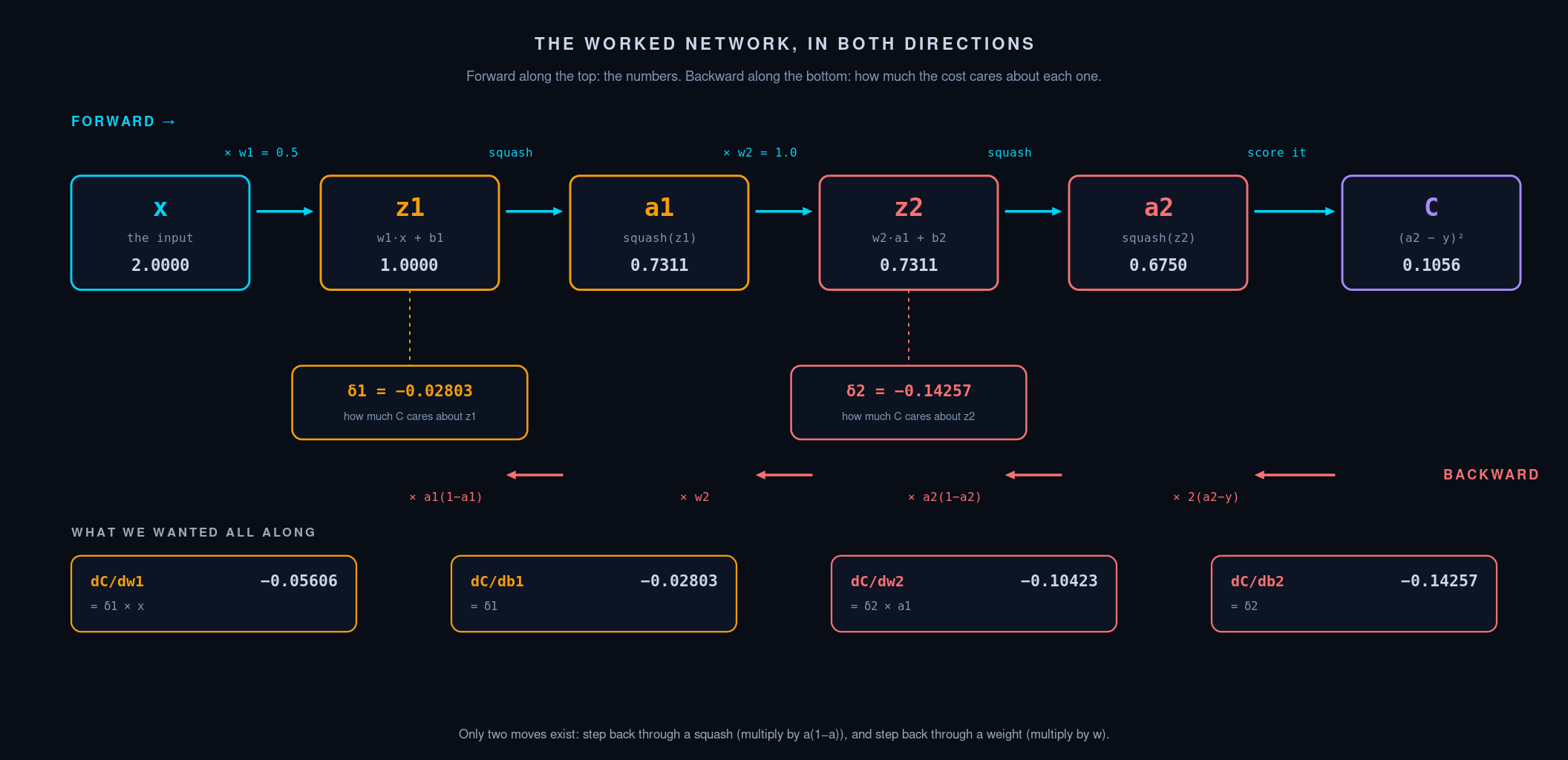
Step 1. \(z_1 = w_1 x + b_1 = 0.5 \times 2 + 0 = 1.0\)
Step 2. \(a_1 = \sigma(1.0) = 0.7311\) (from the table)
Step 3. \(z_2 = w_2 a_1 + b_2 = 1.0 \times 0.7311 + 0 = 0.7311\)
Step 4. \(a_2 = \sigma(0.7311) = 0.6750\) (from the table)
Step 5. \(C = (a_2 - y)^2 = (0.6750 - 1.0)^2 = (-0.3250)^2 = 0.1056\)
The network answered 0.6750. It should have said 1.0. It is wrong, and its wrongness scores 0.1056.
That is the forward pass. Five lines of arithmetic. Nothing has been learned yet — we have only measured the damage.
Part 5 — The backward pass, by hand
Now the real question:
Which of those four numbers — \(w_1\), \(b_1\), \(w_2\), \(b_2\) — should I change, in which direction, and by how much, to make the cost smaller?
We want four derivatives: \(\frac{dC}{dw_1}\), \(\frac{dC}{db_1}\), \(\frac{dC}{dw_2}\), \(\frac{dC}{db_2}\).
We will get them by walking the chain backwards, multiplying rates as we go — exactly the exchange-rate trick from Part 2.
The rates we need at each junction
Before we start, let us write down the rate at each individual step. Each one is easy on its own.
How does the cost respond to the network's answer?
$$\frac{dC}{da_2} = 2(a_2 - y)$$
Derived in Part 1, from expanding a square.
How does a squashed value respond to its input? This is the derivative of the sigmoid, and it has an unusually pleasant form:
$$\frac{da}{dz} = a(1 - a)$$
That is, the output times one minus the output. You do not need to recompute anything — you already have \(a\) from the forward pass. (The algebra is in the box below if you want it; if you do not, verify it by nudging, which we will do in Part 6.)
How does \(z\) respond to its weight, bias, and input? From \(z = wa + b\):
- Nudge \(w\) by 1, and \(z\) moves by \(a\). So \(\frac{dz}{dw} = a\) — the input to that weight.
- Nudge \(b\) by 1, and \(z\) moves by 1. So \(\frac{dz}{db} = 1\).
- Nudge \(a\) by 1, and \(z\) moves by \(w\). So \(\frac{dz}{da} = w\).
Each of those is just reading the equation \(z = wa + b\) and asking what multiplies what. No calculus required at all.
Optional box — where \(a(1-a)\) comes from. Write \(\sigma(z) = (1 + e^{-z})^{-1}\). Its derivative is \(\dfrac{e^{-z}}{(1+e^{-z})^2}\). Now notice that this factorises as \(\dfrac{1}{1+e^{-z}} \times \dfrac{e^{-z}}{1+e^{-z}}\), and that the first factor is \(\sigma(z) = a\) while the second is \(1 - \sigma(z) = 1 - a\). Hence \(a(1-a)\). If that step is not yet accessible to you, skip it — Part 6 confirms the formula numerically, which is arguably better evidence anyway.
Walking backwards
Now we chain. I will do it in the order the algorithm does, from the end.
Rate 1 — cost with respect to the final answer.
$$\frac{dC}{da_2} = 2(a_2 - y) = 2(0.6750 - 1.0) = -0.6499$$
Negative: pushing the answer up makes the cost go down. Which is right — the answer is too low.
Rate 2 — through the final squash.
$$\frac{da_2}{dz_2} = a_2(1 - a_2) = 0.6750 \times 0.3250 = 0.2194$$
Combine them. This gives the single most useful quantity in backpropagation:
$$\delta_2 = \frac{dC}{dz_2} = \frac{dC}{da_2} \times \frac{da_2}{dz_2} = -0.6499 \times 0.2194 = -0.1426$$
\(\delta_2\) (delta-two) means: if the input to the output neuron wobbles by a tiny amount, the cost moves 0.1426 times that, downward. It is the "error signal" at that neuron — and now you know exactly what that phrase means, which is more than most explanations give you.
Now harvest the derivatives at that layer. Both are one more multiplication:
$$\frac{dC}{dw_2} = \delta_2 \times a_1 = -0.1426 \times 0.7311 = -0.1042$$
$$\frac{dC}{db_2} = \delta_2 \times 1 = -0.1426$$
Keep going backwards, into the hidden layer.
$$\frac{dC}{da_1} = \delta_2 \times w_2 = -0.1426 \times 1.0 = -0.1426$$
This is the step that gives backpropagation its name. The error signal has just been passed back through the weight to the previous layer. Notice how it travelled: multiplied by the same weight \(w_2\) that carried the signal forward. Information flows forward through \(w_2\); sensitivity flows backward through the very same \(w_2\).
$$\frac{da_1}{dz_1} = a_1(1 - a_1) = 0.7311 \times 0.2689 = 0.1966$$
$$\delta_1 = \frac{dC}{dz_1} = -0.1426 \times 0.1966 = -0.02803$$
And harvest the first layer:
$$\frac{dC}{dw_1} = \delta_1 \times x = -0.02803 \times 2 = -0.05606$$
$$\frac{dC}{db_1} = \delta_1 \times 1 = -0.02803$$
The whole backward pass on one page
| Step | Formula | Value |
|---|---|---|
| \(dC/da_2\) | \(2(a_2 - y)\) | −0.6499 |
| \(da_2/dz_2\) | \(a_2(1-a_2)\) | 0.2194 |
| \(\boldsymbol{\delta_2}\) | product of the two above | −0.1426 |
| \(dC/dw_2\) | \(\delta_2 \times a_1\) | −0.1042 |
| \(dC/db_2\) | \(\delta_2\) | −0.1426 |
| \(dC/da_1\) | \(\delta_2 \times w_2\) | −0.1426 |
| \(da_1/dz_1\) | \(a_1(1-a_1)\) | 0.1966 |
| \(\boldsymbol{\delta_1}\) | product of the two above | −0.02803 |
| \(dC/dw_1\) | \(\delta_1 \times x\) | −0.05606 |
| \(dC/db_1\) | \(\delta_1\) | −0.02803 |
Ten lines. Every line is one multiplication. That is backpropagation, complete.
Look at the shape of it. There are only ever two kinds of move:
- Step back through a squash: multiply by \(a(1-a)\).
- Step back through a weight: multiply by that weight.
And at each neuron, the running total \(\delta\) is what you multiply by the neuron's input to get the weight's derivative. That pattern repeats identically whether the network has two layers or two hundred.
Part 6 — Prove it to yourself by nudging
You should not believe any of the above. Here is how to check it, and this is the single most valuable exercise in the post.
We claimed \(\frac{dC}{dw_1} = -0.05606\). That claim means something concrete and testable: nudge \(w_1\) up by a tiny amount, and the cost should fall by 0.05606 times that amount.
So do it. Change \(w_1\) from 0.5 to 0.501, leave everything else alone, and run the forward pass again:
- \(z_1 = 0.501 \times 2 + 0 = 1.002\)
- \(a_1 = \sigma(1.002) = 0.731466\)
- \(z_2 = 1.0 \times 0.731466 + 0 = 0.731466\)
- \(a_2 = \sigma(0.731466) = 0.675127\)
- \(C = (0.675127 - 1)^2 = 0.105545\)
The cost went from 0.105601 to 0.105545. It fell by 0.000056.
Divide by the nudge:
$$\frac{-0.000056}{0.001} = -0.056$$
Which is our answer, −0.05606. We derived it with the chain rule; we confirmed it by brute force.
Do this for all four. Using a slightly better method — nudge up and down and take the average slope, which cancels most of the error — here is what you get:
| Parameter | By nudging | By backpropagation | Difference |
|---|---|---|---|
| \(w_1\) | −0.056061 | −0.056061 | 4 × 10⁻⁹ |
| \(b_1\) | −0.028031 | −0.028031 | 5 × 10⁻¹⁰ |
| \(w_2\) | −0.104226 | −0.104226 | 4 × 10⁻⁹ |
| \(b_2\) | −0.142569 | −0.142569 | 9 × 10⁻⁹ |
Agreement to nine decimal places.
This technique has a name — gradient checking — and it is not a toy. It is how people who write neural network code by hand confirm they have not made an algebra error. It is slow, so you would never use it to train anything: checking one parameter costs two full forward passes, so checking a million parameters costs two million. But as a test, it is decisive. If your backpropagation and your nudges disagree, your backpropagation is wrong.
I use exactly this in tinygpt.py, the hand-differentiated transformer behind The Glass Box Transformer. Same idea, 27,861 parameters instead of four.
Part 7 — One step of learning
We now know how the cost responds to each parameter. What do we do with that?
We move each parameter in the direction that reduces the cost.
If \(\frac{dC}{dw} \) is negative, raising \(w\) lowers the cost — so raise it. If it is positive, lower it. In both cases: move opposite to the derivative.
$$w_{\text{new}} = w_{\text{old}} - \eta \times \frac{dC}{dw}$$
The \(\eta\) (Greek eta) is the learning rate: how big a step to take. It is a dial you choose. Take it as 1.0 here, which is large but makes the effect visible.
| Parameter | Old | Derivative | New value |
|---|---|---|---|
| \(w_1\) | 0.5 | −0.05606 | 0.5 − (−0.05606) = 0.55606 |
| \(b_1\) | 0.0 | −0.02803 | 0.02803 |
| \(w_2\) | 1.0 | −0.10423 | 1.10423 |
| \(b_2\) | 0.0 | −0.14257 | 0.14257 |
All four went up, because all four derivatives were negative — the network was under-shooting and every parameter needed to push the answer higher.
Now run the forward pass again with the new numbers:
- \(z_1 = 0.55606 \times 2 + 0.02803 = 1.14015\)
- \(a_1 = \sigma(1.14015) = 0.75771\)
- \(z_2 = 1.10423 \times 0.75771 + 0.14257 = 0.97925\)
- \(a_2 = \sigma(0.97925) = 0.72696\)
- \(C = (0.72696 - 1)^2 = 0.07455\)
| Before | After | |
|---|---|---|
| Network's answer | 0.6750 | 0.7270 |
| Correct answer | 1.0 | 1.0 |
| Cost | 0.10560 | 0.07455 |
The cost fell by 29%. The answer moved from 0.675 towards 0.727, in the direction of the target.
That is learning. Not a metaphor for learning — that is the mechanism, entire. Repeat this loop — forward, backward, nudge the parameters — a few thousand times over a few thousand examples, and you have trained a neural network. Everything else in modern deep learning is refinement of this loop.
A caution worth having early
Notice we took a big step and it worked. It does not always. If \(\eta\) is too large you overshoot the bottom and the cost can bounce or explode; too small and training crawls. There is no formula for the right value — it is chosen by experiment. This is the first place where deep learning stops being mathematics and starts being craft.
Part 8 — When neurons branch: adding up the paths
Our network was a single chain, so each nudge had one route to travel. Real networks branch: one neuron feeds several neurons in the next layer.
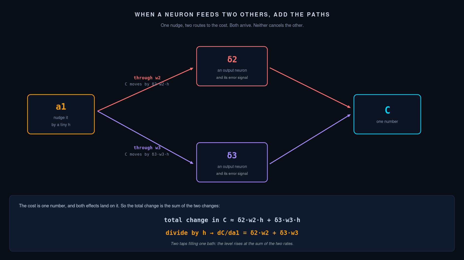
Suppose hidden neuron \(a_1\) feeds two output neurons. Nudge \(a_1\). Its influence now travels down two roads, and both end up affecting the cost.
What do you do? You add them.
$$\frac{dC}{da_1} = \underbrace{\delta_{2} \times w_{2}}_{\text{via the first output}} + \underbrace{\delta_{3} \times w_{3}}_{\text{via the second output}}$$
Why adding is correct, from first principles
This deserves a derivation rather than an assertion.
Nudge \(a_1\) by a tiny \(h\). Two things happen at once, and they do not interfere:
- The first output neuron's input shifts by \(w_2 h\), which changes the cost by about \(\delta_2 w_2 h\).
- The second output neuron's input shifts by \(w_3 h\), which changes the cost by about \(\delta_3 w_3 h\).
The total change in the cost is the sum of the two changes — because the cost is one number and both effects land on it. Divide by \(h\):
$$\frac{dC}{da_1} = \delta_2 w_2 + \delta_3 w_3$$
That is all "summing over paths" means. If a quantity influences the outcome by several routes, add up what arrives by each route. It is the same logic as: if two taps fill a bath, the water level rises at the sum of the two rates.
The general rule
For any neuron in any layer:
The error signal at a neuron is the sum, over every neuron it feeds, of that neuron's error signal times the weight connecting them — all multiplied by the derivative of this neuron's own squash.
In symbols, for neuron \(j\) in some layer:
$$\delta_j = \left( \sum_k \delta_k w_{jk} \right) \times a_j (1 - a_j)$$
That formula is what appears in textbooks, and it typically arrives with no explanation. But you have now derived every piece of it:
- the sum is the branching rule we just derived;
- the \(w_{jk}\) is "step back through a weight";
- the \(a_j(1-a_j)\) is "step back through a squash";
- and \(\delta_j\) is the same running total we computed by hand in Part 5.
When people write this with matrices, the sum becomes a matrix multiplication and the whole layer is done in one line. Matrices are not a new idea here. They are a compact way of writing many of these sums at once.
Part 9 — Build it in a spreadsheet
Now make it real. This takes about ten minutes and it is worth doing, because a spreadsheet recalculates instantly and lets you feel the gradients by changing numbers and watching the cost move.
If you have already done the spreadsheet exercise in Learning With Dr Neal, this will feel familiar — the difference is that there you built the forward pass and let a solver do the learning, whereas here you build the backward pass yourself and can see exactly where every gradient comes from.
Open a new sheet. Column A for labels, column B for values.
The parameters and data
| Cell | Label (col A) | Formula / value (col B) |
|---|---|---|
| 2 | x |
2 |
| 3 | y |
1 |
| 4 | w1 |
0.5 |
| 5 | b1 |
0 |
| 6 | w2 |
1 |
| 7 | b2 |
0 |
| 8 | rate |
1 |
The forward pass
| Cell | Label | Formula |
|---|---|---|
| 10 | z1 |
=B4*B2+B5 |
| 11 | a1 |
=1/(1+EXP(-B10)) |
| 12 | z2 |
=B6*B11+B7 |
| 13 | a2 |
=1/(1+EXP(-B12)) |
| 14 | Cost |
=(B13-B3)^2 |
You should now see 0.675038 in B13 and 0.105601 in B14. If not, stop and find the discrepancy before continuing.
The backward pass
| Cell | Label | Formula |
|---|---|---|
| 16 | dC/da2 |
=2*(B13-B3) |
| 17 | da2/dz2 |
=B13*(1-B13) |
| 18 | delta2 |
=B16*B17 |
| 19 | dC/dw2 |
=B18*B11 |
| 20 | dC/db2 |
=B18 |
| 21 | dC/da1 |
=B18*B6 |
| 22 | da1/dz1 |
=B11*(1-B11) |
| 23 | delta1 |
=B21*B22 |
| 24 | dC/dw1 |
=B23*B2 |
| 25 | dC/db1 |
=B23 |
Check against Part 5: B18 should be −0.142569, B24 should be −0.056061.
The update
| Cell | Label | Formula |
|---|---|---|
| 27 | new w1 |
=B4-B8*B24 |
| 28 | new b1 |
=B5-B8*B25 |
| 29 | new w2 |
=B6-B8*B19 |
| 30 | new b2 |
=B7-B8*B20 |
Now train it
Copy B27:B30, then paste-special-as-values into B4:B7. Every cell recalculates, and the cost in B14 drops.
Do it again. And again. Watch B14 fall: 0.1056 → 0.0746 → 0.0546 → and onwards towards zero. Watch B13 crawl towards 1.
You have just trained a neural network in a spreadsheet, by hand, with no code.
Three experiments worth doing
- Set the rate (B8) to 10. Does it learn faster, or does it thrash? Try 50.
- Set
yto 0 instead of 1 and retrain. All the derivatives flip sign and the network learns the opposite answer. - Break the backward pass on purpose — change B22 to
=B11(dropping the \((1-a_1)\)). Train it. It still improves, just worse. This is why a plausible-looking bug in backpropagation is so dangerous: the network still learns something, and only a gradient check catches it.
That third one is the most instructive. It is exactly why the nudge test in Part 6 matters.
Part 10 — Why backwards?
We have never justified the direction. Why not start at the weights and work forwards?
You could. It gives the same answers. It is just catastrophically slower, and understanding why is understanding why this algorithm exists at all.
Forwards: to find how \(w_1\) affects the cost, you push a nudge in \(w_1\) through every subsequent layer to the end. Then to find how \(b_1\) affects the cost, you do the whole journey again. Then for \(w_2\). Each parameter requires its own full sweep of the network. With a million parameters, that is a million sweeps.
Backwards: you start at the cost and sweep back once. At each neuron you compute \(\delta\) — and that single number is then shared by every weight feeding into it. Nothing is computed twice.
The saving is enormous and it is the reason deep learning is possible at all. A modern network has billions of parameters. Backpropagation gets the derivative of the cost with respect to all of them for roughly the cost of two forward passes. The forward-mode alternative would need billions.
This is the same reason we work backwards through a chain in Part 5: the front of the chain is shared by everything behind it, so compute the shared part once and reuse it.
Part 11 — What is different in a real network
Everything above is complete and correct. Here is what changes at scale — and the answer is: less than you would think.
Many neurons per layer. Layers become vectors, weights become matrices, and the sums of Part 8 become matrix multiplications. The rule per neuron does not change.
Many layers. Repeat "step back through a squash, step back through a weight" more times. The chain is longer; the links are identical.
A different squash. Sigmoid is rarely used in hidden layers now. ReLU — "if the input is positive, pass it through; otherwise output zero" — is standard, and its derivative is even easier: 1 where the input was positive, 0 where it was not. Substitute that for \(a(1-a)\) and everything else stands.
A different cost. For classification, squared error is replaced by cross-entropy. Only the very first step of the backward pass changes — the \(\frac{dC}{da}\) term. The rest of the machinery is untouched.
Many examples at once. Real training averages the gradient over a batch of examples before stepping. Compute the derivatives for each example, average them, then update once.
Cleverer steps. Plain gradient descent is rarely used unmodified; optimisers like Adam adapt the step size per parameter based on recent history. They change how far you step, never how the derivative is computed.
Automatic differentiation. In PyTorch or JAX you never write any of this — the framework records what you did on the forward pass and replays it backwards. But it is doing precisely what you just did by hand. Which is why doing it by hand once is worth a great deal: when the framework produces something strange, you know what it was trying to do.
Part 12 — Things that confuse people, answered
"What is being propagated backwards, exactly?" Sensitivity. Specifically, \(\delta\) at each neuron: how much the cost would change if this neuron's input wobbled. Not error, not blame — a rate of change.
"Why does the derivative use \(a\) rather than \(z\) in \(a(1-a)\)?" Convenience, nothing more. The derivative genuinely depends on \(z\), but for the sigmoid it happens to be expressible using the already-computed \(a\). Saves recomputation. Other activations are not always so kind.
"Where did the bias derivative go? It is just \(\delta\)." Because \(\frac{dz}{db} = 1\) — nudge the bias by one, and \(z\) moves by exactly one. Multiplying by 1 leaves \(\delta\) unchanged. The bias derivative is the error signal.
"Why is \(\frac{dC}{dw} = \delta \times \text{input}\)?" Because \(z = w \times \text{input} + b\), so nudging \(w\) by 1 moves \(z\) by the size of the input. A weight receiving a large input has more leverage on the outcome, and so gets a larger derivative. This has a real consequence: a neuron that outputs near zero barely trains the weights it feeds.
"My network trains but badly. Is my backprop wrong?" Run the nudge test from Part 6. It will tell you in one minute, definitively. As experiment 3 in Part 9 shows, broken backpropagation often still learns — just worse — so "it seems to be working" is not evidence.
"Do I need to understand this to use PyTorch?" No. You should anyway. Nearly every hard training bug — vanishing gradients, dead neurons, exploding losses — is a statement about what is happening in the backward pass, and is close to unreadable if you have never seen one.
What to do next
If you did the spreadsheet, you now understand backpropagation better than someone who has read ten articles about it, because you have made the numbers move.
Two things worth doing:
Widen the network. Add a second hidden neuron to your spreadsheet. You will need the summing rule from Part 8 for \(\frac{dC}{da_1}\). It is fiddly rather than hard, and it is where the general formula stops being abstract.
Watch 3Blue1Brown. Grant Sanderson's visual treatment complements this one exactly — where this post is arithmetic you can check, his is geometry you can see. Chapter 3 builds the intuition for what backpropagation is doing; Chapter 4 does the calculus, and if you have worked through this post you will recognise every step of it. Do them in that order.
Sources and further reading
- 3Blue1Brown — What is backpropagation really doing? (Deep learning, chapter 3) — the intuition, visually. Also on 3blue1brown.com.
- 3Blue1Brown — Backpropagation calculus (Deep learning, chapter 4) — the same material in symbols, and the clearest short treatment of the chain rule in this setting. Also on 3blue1brown.com.
- The Glass Box Transformer — everything in this post, scaled up to a complete language model with every gradient derived by hand.
- tinygpt.py — the code for that, including the gradient check from Part 6, in about 480 lines of NumPy with no framework.
All numbers in this post were computed and independently verified against numerical gradients; the two agree to roughly nine decimal places. If your arithmetic disagrees with mine, I would like to know.